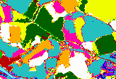
Fig 1: Example of input image
Algorithm of vectorization of aerial classified images
Jaroslav Fojtík
Czech Technical University, Faculty of Electrical Engineering
Centre of Machine Perception
121 35 Prague 2, Karlovo náměstí 13, Czech Republic
telefon +42 2 24357465, FAX +42 2 290159
E-mail:fojtik@cmp.felk.cvut.cz
currently: fojtik@htc.honeywell.cz
Abstract: This work describes transformation of raster data into the vector representation. The work focuses to the description of algorithm. Most of current works about automatical vectorization, that I could meet, was based on the usage of existing software package. Authors of these tools usually do not share used algorithms. Thus is was designed new algorithm according to specification from company Help Service. This algorithm is good for vectorization of aerial images. Input image must be preprocessed by domain detector.
Cartographists attempts to maintain actuality of theit maps. So grabbing of new aerial images of landscape is done. Old maps are actualised according to resulting snapshots see[6]. This type of work is currently done manually or semiautomatically with using ready to use programs. The task of author is to explore possibilities of algoritmization of separate steps duting conversion from aerial image into the bitmap. The result should be saving of human work during creation of maps from aerial images.
Currently available methods of vectorization do not gave us acceptable results, or the description of algorithm was not available see [3,8,9,12]. Therefore it was designed and realized new approach based on the topology of finite spaces.
Processing of aerial image consists from these steps:
The vectorization algorithm is designed for searching boundaries of continuous areas. There should exist homogenous areas with same labeling (represented by color it means by number written as pixel value). Each labeling represents crucial property of input data. For example wood, lake, road etc. Found boundaries of areas are transformed into vector representation.
Fig 1: Example of input image
This algorithm isn't designed for finding edges in gray-scaled image. For this it must be first preprocessed. After preprocessing can algorithm continue from 2nd step see below. For preprocessing any edge detector can be used eg Canny see[1], and its output (after tresholding with hysteresion) could be translated by described approach into the vector representation.
The basic of simple vectorisation methods is discused in this chapter. They produce output bitmap with the same size as input bitmap and they ignore topological problems at all. Similar method was implemented in the GIS TopoL.
The whole image is traversed using operator, which tests equality of values two adjacent pixels. Equality is tested in all 8 neighborhood directions of actual point (may be 4 neighborhood too). If inequality occurs in one or some directions together, then output pixel is set to 1. Otherwise it is set to 0. The behavior of operations is shown in following images Fig2 a Fig3.
 |
 |
|---|---|
| Fig 2: Original bitmap | Fig 3: Bitmap after vectorization |
This process has essential disadvantage to double response for each edge. Of course there exists improved variants which tests equality only in some directions e.g. only from right to left and from up to down. This way is able to partially compensate double response but not absolutely. Problems approves around occurrence single point which lays on any other edge. Moreover all edges will be shifted in some direction.
Previous problems are caused by incorrect representation of boundaries. This representation was used in oldest TopoL releases. Therefore results of topology of finite spaces are used [14].
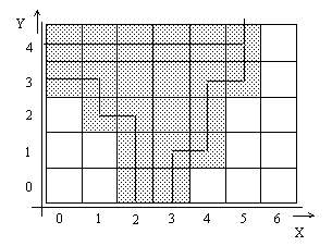
The original bitmap isn't too advisable for searching of boundaries see Fig 4 and their positioning. Therefore the new method was used, which guarantee much better quality of detected edges.
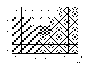
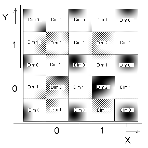
New pixels are added to the original bitmap at corners and on edges of original pixels see Fig 5. These new points have special properties and are used for expressing of topological relations among image data. Procedure of extension is graphically shown on series of figures Fig 4-6.
 |
 |
 |
|---|---|---|
| Fig 4: Original image | Fig 5: Celuar complexes | Fig 6: New representation |
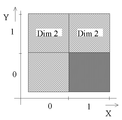
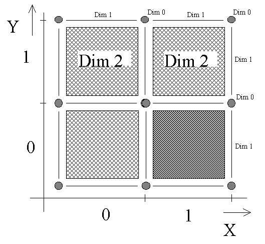
Final bitmap is depicted on Fig 6. It is extended by new pixels. These pixels describes edges of the pixels and corner points. The paradox of two lines doesn't arise in this configuration see[1 page:30].
Original pixels are preserved and they represents elements with dim (dimension) 2. Edges of two pixels have dim 1 and elements in corners have dim 0.
From these presumption follow following constraint. The edge as 1 dim unit must not pass through points with dim>1, is should only pass through points with with dimension <=1. The branching of edge (node) might occur only in the point with dim=0, it means in the corners of pixels.
The design of algorithm is modular.
Used approach is very modular. For example if the requirements change only several modules could be replaced. For example if the another GIS will be used, only the last 5th module should be replaced. Each module realises one pass. Vectorizer has 5 main passes. Only bitmap data are processed during first two pasess. The vector representation is build during 3rd pass and last 2 passed manipulates only with vector representation.
Original image has a size [x;y].
1st .Pass - finding edges
Edges of domains are finded in this pass. It is constructed new auxiliary binary raster (in the current implementation it is named KDT.RAS) with sizes [2*x+1;2*y+1]. Its borders are set into value 1. Insideous points are set only if condition, that lies between two points with different level of brightness. It is evaluated differences in longitudal, lateral and diagonal directions.
Following two tables shows this process of bitmap transformation.
| Original image: |
| Is transformed to: |
|
(Only dot signed '.' points are stored in bitmap - value 1 other points has value 0. The numbers are inserted only for highlighting the correspondence with the previous image)
2nd Pass - finding of nodes Nodes are detected in this pass. Second auxiliary binary raster of nodes (in the current implementation it is named KDU.RAS) with sizes [2*x+1;2*y+1] is constructed. A node is such point, which has more than two nonzero neighboring points. For node detection is used binary operators similar of that used for dilatation.
| Thus our image is transformed to: |
|
(In bitmap there are stored only points signed using character 'x' = value 1 other points has value 0. The dot points are inserted only for highlighting the correspondence with the previous image)
3rd Pass - detection of the vector lines;
In this pass are calculated vector lines. Each vector line must rise from any node and lead into any (may be other) node. Next 3 auxiliary files (that are in current implemantation named POINTS.BIN, NODES.BIN and LINES.BIN) are constructed. Checking of lines runs following way: The bitmap KDU.RAS is sequentially traversed until a first node is found. From this node is tried to go out (trace lines) to all four directions. In process of tracing line are found neighboring and these are signed into internal structure. In this process are points by sequel erased from auxiliary raster KDT.RAS Line tracing process finishes when node point is found. Then line is represented by list of vertexes. The count of vertexes is optimized by special algorithm. It is based on the least square criteria that is calculated from deviation optimized broken line from original one.
Algorithm described in the Pass 3 isn't abbe to find closed circles without nodes. Thus 3rd pass is executed twice. In 2nd process is any found point (in the raster KDT.RAS) considered as node point (with order 2) and all circle is found (and erased) by sequential pass. (Please keep in mind that all other was already erased from raster KDT.RAS !)
There are no longer needed rasters KDU.RAS and KDT.RAS erased at the end of this pass.
4th Pass - checking areas
Closed areas are searched from each node point. Progress of searching begins in node, it continue through the line and next node point. After this the progress continues clockwise until beginning node is reached. From specification (in respect of previous steps) follows, that graph must be planar. Above specified procedure must every time generate closed circle.
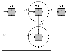
Example of scanning progress (according to Fig. 7):
Let U1 is a start point and let socket 1 points to the valid line. Searching continues along the line L1 to the node U2. Input direction in U2 is realized through socket No 3. First clockwise found socket with line has No 4. This socket will be used for leaving node U2. Scanning goes out from node U2 along line L3 into next node U4. Input socket in U4 has No2. First clockwise found socket with line has No 1. Output line L4 returns to start node. The area is closed at this point and the algorithm finishes.
When going around the area its size is counted. If is greater then limit, then all lines belonged to mentioned area are marked as valid (flag is placed in node points).
In node points are also stored all informations about progress. This ensure only one scanning of each area and no area is accessed twice.
5th Pass - building topological structure
It is traversed by nodes like in the previous example. All nodes are checked. In each node are hitherto unerased lines topologically joined together.
The so called gluing lines is made in this pass. Last 2 valid lines lines that goes from one node could be glued because of its neighborhood lines was already erased in the previous pass and degree of node decreases into value 2. Each node with degree 2 (in each circle must one left) is found and erased from graph. When the lines are created the areas are generated. The topology will not change, but the amount of output data will be significantly decreased. Found and corrected lines are exported into internal structures of GIS TopoL. Only this step is dependent on the used GIS.
At the end of this pass are in future unneeded files LINIE.BIN, BODY.BIN and UZLY.BIN erased.
V této kapitole je obsažena diskuse o nastavitelných parametrech a jejich vlivu na výstupní vektorový formát.
Program has at all 5 parameters:
a, Name of the input file.
b, Name of the output block.
c, Minimal accepted size of the area.
d, Deviation vector line from raster.
e, Switch for rejecting border areas.
a, Input image may by in any type 2,16,256 brightness levels (with or without palette), DMT or true color (this constrain stems from used package TopoL). But it must contain continuous domains with equal brightness value.
b, The name of output block specifies the path (of block directory), where output data will be stored. Destination device must have enough free space for storing temporary data.
c, Minimal size of the area is measured in pixels (if somebody wish may be converted into Ha). If it is too small <1,10> pixels, then the size of output vector image might extremely grow.
d, Deviation of vector line indicate even of vector line and this parameter schedule a number of removed redundant vertexes. Unit of its value is point/point of line. The values from range 0.1 to 0.9 are recommended. If this value is too small, then output lines are not smooth. If this value is too big, then the shape of areas are deformed.
e, If the switch of border areas is set, then in output image will be areas which touches border of the image. In another case are areas mentioned above ignored and removed from output file.
The length of output vector file is discused in this chapter. It is clear that vector format is another representation of data. The vector size could be larger than original raster one, when the precision requirements are very high and for some special types of rasters. More data in the vector representation compensate much greater comfort during editing and during changes.
Let us have chessboard its size of domain 8x8 (it means 64 points). This case is near worst possible.
Each field (domain) will be on output one area. Each domain have 4 lines. Lines are shared with neighbor cells. Required precision of vectorization is maximal.
Next calculations concerns to data sizes of TopoL package, but obtained results could be applied also for another vector representations:
Length of line = 103 bytes + 2 outer points 24 bytes (4x6)
Length of area = 71 bytes
Lpl = 4*(103+24) /2 + 71 = 325 byte
Lpl is a count of bytes needed for one domain of chessboard in vector format. Original size of each domain in raster representation was 64 bytes (for 256 colors), or 32 byte for 16 colors. It mens that length of data increases 5 (or 10) times.
Vector format is space saving (output data size) from minimal size of area 325 points, it corresponds to the minimal field size 18x18. It the size of area is 1 then the size of vector image may be 300x larger than that original raster image.
User must carefully weigh the price of details that he needs to have in output vector data (or have sufficient space on destination disk).
In this paper described method of automatic vectorisation is able save much work to peoples, whom later must do manually the vectorisation of aerial images manually or semiautomatically. The current implemantation is able to process very large images about hundreds Mb. It is currently a part of GIS package TopoL. User must have enough free space on disk and became familiar influence of input parameters to requirements of his particular task.
Fig 8: Output of vectoriser for image Fig 1
[1] Václav Hlaváč, Milan Šonka. Počítačové vidění. Grada 1992.
[2] Rik D. T. Janssen, Albert M. Vossepoel Adaptive Vectorization of Line Drawing Images
[3] Emil Ryník. Tvorba vektorovej kastrálnej mapy vo východoslovenskom regione. Geodetický a kartografický obzor, ročník 82/84 1996, č 11, str 227-229.
[4] K.-J. Schilling, T. V"gtle. Satellite Image Analysis using Integrated Knowledge Processing. ISPRS vol XXXI, part B3, Vienna 1996 (752-757)
[5] Vít Zýka. Inteligentní interpretace vektorových dat. Diplomová práce ČVUT FEL 1996
[5] F. Kressler K Steinnocher. Change Detection in Urban Areas Using Satelite Images and Spectral Mixure analysis. ISPRS vol XXXI, part B7, Vienna 1996 (379-383)
[6] Saeid Noori Busheri, Nooshin Khorsandian. Improved Classification of Spot Multi-Spectral Images for Land Cover Evaluation Assisted by Digital evaluation Model (DEM) and Aerial Photographs. ISPRS vol XXXI, part B7, Vienna 1996 (534-541)
[7] Aleksandra Bujakiewicz. Simple Photogrammetric Methods for Mapping of Vegetation Polygons Boundaries in National Parks in Africa. ISPRS vol XXXI, part B4, Vienna 1996 (154-158)
[8] Viktor Latejčuk, Adri na Treščáková. Tvorba VKM v katastrálnom odbore v Michalovciach. Geodetický a kartografický obzor, ročník 48/84 1996, č 12
[8] Oldřich Kafka. Automatizace obnovy map katastru nemovitostí. Geodetický a kartografický obzor, ročník 41/83 1995, č 8
[9] Dagmar Kusendov , Martin Kamenský. Objektovo-topologická digitalizácia máp. Geodetický a kartografický obzor, ročník 39/81 1993, č 8, str 166-170
[10] Adolf Vlajča. Problémy digitalizace souboru geodetických informací katastru nemovitostí. Geodetický a kartografický obzor, ročník 40/21 1994, č 6, str 119-125.
[11] Ján Feranec, Ján Oťaheľ, Marcel Šúri. Mapovanie vegetácie pomocou leteckých farebných infračervených snímok GIS-u SPANS.
[12] PeterG.M.Mekenkamp. Global changes and GIS-Accuracy. XX Congress Melbourne, Australia, commision 3, str 102-111
[13] Giles M. Foody. Cross-entropy for the evaluation of the accuracy of a fuzzy land cover with fuzzy ground data. ISPRS Journal of Photogrammetry and Remote Sensing, Num 5, Vol 50, Septempber 1995
[14] Kovalevsky V. Digital geometry based on the topology of abstract cell complexes, Conference in France, 1993, strany {259--283}.
Please cite this paper as:
Jaroslav Fojtik. Algorithms of vectorisation aerial images.
In Institut of economy and control systems HGF VSB
TU Ostrava, editor, GIS Ostrava 98, pages 102-110, Ostrava-Poruba VSB TU,
January 26-28 1998. Mining university - Technical University.